To navigate this multi-page article:

Use the drop-down lists and arrow icons located at the top and bottom of each page.

 

Figure 1: Trapezoidal Storage Tank (click for 3D)

We turn now to some tasks for which Sage is very well suited. This page is meant to show what Sage can do, but it also describes the solution to a practical problem — determining the volume of liquid contained in an odd-shaped but common storage tank, for different sensor measurement heights.

The page following this one addresses tanks with a circular cross-section. That class of tank has a somewhat more complex volume computation, so I thought I would first describe a kind of flat-sided tank with a comparatively simple solution.

In reading this article it will benefit the reader to have access to a Sage notebook interface, either locally or online. To get your free copy of Sage, click here.

(Click here for a Sage worksheet with resources used in this page.)

Refer to Figure 1 on this page. A tank like this might have sides all parallel/orthogonal (a cube), in which case the total volume is equal to x * y * z, and a partial volume equal to x * y_sensor * z, with y_sensor referring to the liquid sensor height in the tank. Unfortunately, there are few real-world tanks with parallel sides.

A tank that I describe as "first-order trapezoidal" has one non-parallel dimension (a dimension whose enclosing sides are not parallel). The tilted side might lie in the x or z dimension, but its key property is that it isn't parallel with the opposite side of the tank. The full volume of such a tank is not at all difficult to compute:

(1)   

Where x_b and x_t are the tank widths at the bottom and top of the non-parallel dimension, and y and z are the sizes of the two parallel dimensions.

Figure 2: Old-style linear regression

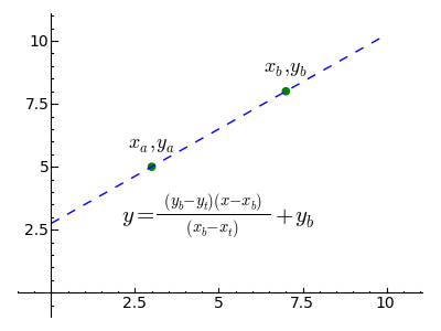
Figure 3: Computer-based linear regression

Interpolation

We turn now to the first non-trivial computation. For the above first-order trapezoidal tank, we need a way to compute the volume of the tank's liquid contents for any arbitrary sensor height in the y (vertical) dimension. We know the width of the tank at the bottom and the top, but to compute partial volumes we need to find intermediate tank widths for any sensor height, and then apply a version of equation (1) above. To be more specific, we need to way to interpolate between x_b and x_t as a function of the y dimension sensor height.

The classic procedure for acquiring a linear regression is shown in Figure 2. This method was common at a time when computations were performed by hand, using pen and paper and possibly a slide rule or an abacus. Because of these constraints, the procedure was broken down into as many steps as possible to guard against error.

Now that computers are ubiquitous, a more flexible, one-step regression equation is becoming popular. Shown in Figure 3, it is normally embodied in a function for convenience and so that its users are not burdened by its inner workings (a computer science idea known as "encapsulation").

Let's start a Sage session and create a cell at the top of the worksheet with this initializing content (those in a hurry can click here to get a copy of my worksheet for this article):

#auto
reset()
var('m b v x y z a b c d x_a x_b x_t y_a y_b y_t z_b z_t')
# special equation rendering
def render(x,name = "temp.png",size = "normal"):
    if(type(x) != type("")): x = latex(x)
    latex.eval("\\" + size + " $" + x + "$",{},"",name)
def radians(x):
    return x * pi / 180
            

Remember when copying and pasting these complex cell contents: resist the temptation to "fix" the indentation of certain lines. The indented lines must remain as shown for the content to work as intended.

Now let's create a Sage interpolation equation/function:

# interpolation function
ntrp(x,x_b,x_a,y_b,y_a) = (x-x_a)/(x_b-x_a)*(y_b-y_a)+y_a
render(y == ntrp(x,x_b,x_a,y_b,y_a),"ntrp.png","Large")
            

(2)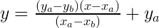   

The reader can see from this example that the custom function "render(x)" produces a nice graphic rendering of its argument, suitable for exporting into a Web page like this one. Readers who want to use this function need to understand that the graphic image displayed in the Sage worksheet won't be automatically saved anywhere useful — the user must right-click the image, click "Save Image As..." and specify a path.

Some readers may wonder why I have written ntrp(x,x_b,x_a,y_b,y_a) as a pure mathematical function rather than a Python function (as I did for the function "render(x)" earlier). The answer is that if one intends to use the function in algebraic manipulations, the pure mathematical function form is needed, but if processing speed is the only issue, a Python function is preferred. As it turns out, this function will be used as a component in a number of increasingly complex equations later on, and its ability to encapsulate the idea of interpolation while hiding its gory details greatly simplifies the expressions in which it is used.

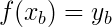
Before we go on, let's test the interpolation function. I rarely write such a function without testing it, regardless of how self-evident it may seem. The function has the property that it will accept an argument expressed in terms of x_a and x_b and translate it into a range corresponding to y_a and y_b, so that:

(3)   

and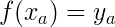

(4)   

and that intermediate x arguments produce a linear range of intermediate and proportional y results. But mathematical ideas like this, even when self-evident, are not easy to express in words. Here is a clearer way to say it:

print "<html><u>  &deg;c   &deg;f </u></html>"
for c in range(0,110,10):
    print "%4d %4.0f" % (c,ntrp(c,100,0,212,32))
            

  °c   °f 
   0   32
  10   50
  20   68
  30   86
  40  104
  50  122
  60  140
  70  158
  80  176
  90  194
 100  212
            

First-Order Trapezoidal Volume

Now let's create a function to provide intermediate volumes for our first-order trapezoidal storage tank. To accomplish this we'll be using an idea from Integral Calculus — if we write a function that provides the (x,z) cross-sectional area of an imaginary slice through the tank at a given height y, we can get a partial volume by integrating the area function between the bottom of the tank and any provided height argument. Here is an area function for this type of storage tank:

# first-order (x) trapezoidal tank area
fax(y,x_t,x_b,z,y_t,y_b) = ntrp(y,y_t,y_b,x_t,x_b) * z
render(a == fax(y,x_b,x_t,z,y_b,y_t),"fax.png","Large")
            

(5)   

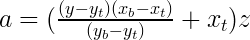
Notice that, instead of trying to rewrite the interpolation function to apply it to this case, I simply entered variable names appropriate to this example and let Sage sort it out. (The variable subscripts refer to their position on the tank: x_b = bottom, x_t = top.) Because the size of this tank's z dimension is a constant, to get an area I simply multiply the interpolation result by z.

How difficult will it be to create an integral of this area function, in order to acquire intermediate volumes? Well, it's not difficult at all:

# first-order (x) trapezoidal tank volume
fvx(y,x_t,x_b,z,y_t,y_b) = integrate(fax(y,x_t,x_b,z,y_t,y_b),y)
render(v == fvx(y,x_t,x_b,z,y_t,y_b),"fvx.png","Large")
            

(6)   

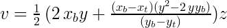
In order to keep this article from becoming overly large, I'm going to move ahead to the more generally useful second-order trapezoidal solution, which can be made to compute this tank type also (by setting z_b and z_t to the same value).

Second-Order Trapezoidal Volume

Let's use the same procedure for this tank type — let's create a function that will produce a surface area at any content height y, then integrate to get a volume. Remember about this tank type that there are two non-parallel dimensions (x and z) so for an area calculation we need to interpolate twice and multiply the interpolation results together. Like this:

# second-order (x,z) trapezoidal tank area
faxz(y,x_t,x_b,z_t,z_b,y_t,y_b) = ntrp(y,y_t,y_b,x_t,x_b) * ntrp(y,y_t,y_b,z_t,z_b)
render(a == faxz(y,x_b,x_t,z_b,z_t,y_b,y_t),"faxz.png","Large")
            

(7)   

Now let's take the integral of our area function:

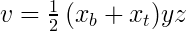
# second-order (x,z) trapezoidal tank volume
fvxz(y,x_t,x_b,z_t,z_b,y_t,y_b) = integrate(faxz(y,x_t,x_b,z_t,z_b,y_t,y_b),y)
render(v == fvxz(y,x_t,x_b,z_t,z_b,y_t,y_b),"fvxz.png","Large")
            

(8)   

Scroll horizontally to see the full result. This time we'll be testing our function before putting it into service in a field where, because of what these storage tanks might contain, there is no such thing as a trivial wrong result.

First, let's specify the arguments needed for the second-order volume integral. They are:

(9)   

Where:

• x_b, x_t = x dimension bottom and top widths.
• z_b, z_t = z dimension bottom and top widths.
• y_b, y_t = y dimension heights corresponding to the x and z widths.
• y = sensor height within tank.
• v = tank partial volume for sensor height y.

First test (trivial): We know the full volume of an ordinary, parallel-sided tank should be x * y * z, and this function should produce this result if given the appropriate arguments. Let's test it:

fvxz(10,10,10,10,10,10,0)

1000

This entry describes a tank with x and z top and bottom dimensions the same, and a y height of 10 units. A cube 10 units on a side has a volume of 10³ = 1000, so this result is correct. Now let's create a first-order result by specifying half width at the bottom of the x dimension:

fvxz(10,10,5,10,10,10,0)

750

We know this is right — if divided in half diagonally, the tank would have a volume of 10³/2 = 500, and by specifying x_b = 5 and x_t = 10 this example removes half that volume, so a result of 750 is correct.

Tests that change both the width and depth of the tank are not so easy to interpret, but there is an exception — a pyramid, which should have a volume of x * y * z / 3. Here is how we describe a pyramid:

fvxz(10,0,10,0,10,10,0)

1000/3

This entry describes an object with zero width at the top in both the x and z dimensions, a bottom width of 10 units for x and z, and a y height of 10 units, e.g. a pyramid. The result is correct.

Computer scientists are familiar with the idea of solving subproblems, encapsulating the solutions, then moving to higher levels of abstraction using the prior solutions as components. It happens this is an effective tactic in applied mathematics as well, but until now mathematicians haven't had a practical way to encapsulate and reuse (except in an abstract sense with few tangible manifestations). Programs like Sage offer an opportunity to practice mathematics in a very productive way, building solutions piecemeal by writing and testing comparatively simple elements, then solving larger problems by assembling such elements in combination.

In this example problem we created a relatively simple interpolation function, tested it, then applied it to the solution of a more complex problem. Sage allowed us to use our function in expressions that were easy to understand, then presented its results in classic equation form.

This page also serves as a resource for people in the storage tank business, it isn't just a Sage tutorial. It's my hope that it will motivate storage tank operators to adopt Sage or another similar computer algebra system to solve their tank calculation problems.

Equation Simplification

Those having experience with Sage will notice I haven't applied "simplify()" or "simplify_full()" to my equations on this page. I haven't because at the time of writing (Sage version 4.1.2) "simplify()" and related functions aren't particularly effective and sometimes perversely make an equation larger, an issue to which I shall return.

Equation Rendering (rant)

I created the custom equation rendering function "render()" out of necessity — there are few effective ways to take an equation from a computer algebra system and place it in a Web page. There's MathML, an ambitious project meant to allow math rendering in Web pages. Unfortunately this project is almost as complex and ineffective as it is ambitious. There's TeX, which has a loyal following in academia, but it isn't a particularly efficient way to put an equation in a Web page (my function "render()" ultimately relies on TeX to get its results).

I had originally intended to put a cross-reference table here, showing those CAS programs that were willing to accept plain-text versions of equations created by the others. But I quickly discovered there is essentially no present way to transfer an equation from one environment to another — Mathematica, Sage, Maxima, Maple, TeX, the OpenOffice Math equation editor and the Microsoft Word equation editor all use mutually incompatible equation syntax. At one time it was hoped that TeX would become the lingua franca for mathematical equation rendering, unfortunately TeX lives in a world of its own and rarely condescends to visit this one (a truly baroque procedure is required to turn TeX syntax into a graphic).

Portable math equation rendering is an unsolved problem at the time of writing. The drawbacks to a set of graphic images of equations (as in this article) become obvious when one scales the page up for easier reading. And the size of the graphic equations rarely matches the surrounding text.

MathML might eventually be adopted, but only after the committee responsible for it stops releasing new versions that summarily invalidate the old. My impression of MathML was recently confirmed when I tried to use its methods in a page I was designing. I couldn't get the simplest example to work, even when I copied a self-contained example from one page to another. I finally realized the only difference between the pages was the file extension — "xhtml" in the original and "html" for my experimental file (identifying the page's content as XHTML within the page had no effect). I realized to adopt MathML I would have to rename all 625 of my HTML pages and invalidate tens of thousands of worldwide links that refer to my pages, all in order to render equations more efficiently.

  "Exploring Mathematics with Sage" by Paul Lutus is licensed under a
Creative Commons Attribution-Noncommercial-Share Alike 3.0 United States License.