

 Share This Page
| Home | | Mathematics | | * Applied Mathematics | | * Storage Tank Modeling | | | | Share This Page |
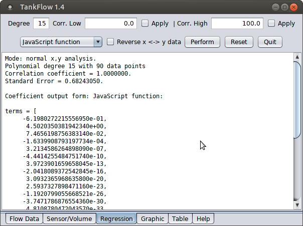
Figure 1: Polynomial regression result |

Figure 2: Storage tank height/volume profile (click for full-size) |
TankFlow is a powerful flow-based storage tank analyzer.
Copyright © 2019, Paul Lutus — Message Page
Latest TankFlow Version: —
Most recent update to this page:
Figure 3: Pathologically shaped tank
TankFlow produces storage tank volume profiles, a central issue in the use of storage tanks. There are a number of ways to profile a storage tank, some easy, some difficult. TankCalc, another of my programs, models a tank using geometry — if a tank's dimensions are known and not pathological, geometry is a relatively easy way to create a height/volume profile (see Figure 2) that associates the tank's sensor readings with its volume.
TankFlow uses a different approach — it requires that the tank be filled in a controlled way, while recording times, flow rates, and content sensor heights, then it performs some mathematics to create a profile.
Again, if a tank has known, normal geometric dimensions and no internal irregularities, then TankCalc is a better approach — it's simpler and less labor-intensive. But if a tank has internal obstructions, is oddly shaped, is buried or is otherwise inaccessible, and for whatever reason cannot be described in simple geometric terms, then TankFlow may be a better approach.
TankFlow is © Copyright 2019, P. Lutus, is licensed under the the GPL, and is free.
TankFlow has several available download packages, depending on the user's system requirements:
- A Windows installer package.
- An executable Java JAR file, for use on platforms other than Windows.
- A source archive organized as an Eclipse project.
TankFlow is written in Java and therefore requires a Java runtime engine available here.
Here is a link to a local copy of TankFlow's built-in help page.
For this kind of analysis, the central (and most difficult) activity is a manual fill profile of the storage tank — everything else relies on an accurate fill and data collection. Here's an outline of the process:
- Acquire a good source of elapsed time — a modern watch with a display of seconds meets this requirement.
- Use the most accurate available flow-meter to measure the rate at which content flows from the source tank to the measured tank. This accuracy requirement cannot be overemphasized — if the flow meter is in error by 10%, the tank's resulting volume profile will have the same error.
- Arrange to measure the tank's content height in the most accurate possible way.
In this activity, periodic records are made of the time (to the second if possible), the pumping flow rate and the tank content sensor height. At the end of the process, there should be enough records to accurately profile the tank — 100 such records is not too many. This means if two hours are required to fill a tank, measurements should be taken each two minutes or less.
The exact time between measurements is not important, as long as the time is accurately recorded, and as long as plenty of data points are recorded. The data can be entered onto a paper tablet (to be later transcribed into a computer text file), or into a spreadsheet (preferable) or a plain-text file. Each record looks like this:
13:22:41, 100.24, 324.77
- Each record should appear on a separate line in the text file (or spreadsheet) and have three fields, as shown.
- The first field is the time of day — it should include hours, minutes and seconds if possible. Keep this entry simple, don't include AM/PM or other regional time notations — just hours:minutes:seconds.
- The second entry is the flow rate at the time the measurement was taken. Always record the flow rate for each measurement, don't assume the rate will remain the same.
- The third entry is the tank content sensor height, measured as accurately as possible.
For maximum measurement accuracy, use a source tank that's larger than the destination tank — this avoids large changes in flow rate as the destination tank fills.
Once a text file (or spreadsheet) has been populated with field measurements, it's time to let TankFlow perform an analysis and create a profile.
For simplicity TankFlow uses the system clipboard for data transfers. All data that's imported and exported to/from TankFlow, goes by way of the system clipboard.
Here's how to import field measurement data into TankFlow:
- Run the spreadsheet or text editor program that has the measurement data collected earlier.
- When the data are on display, press Ctrl+A (PC) or Command+A (Macintosh) to select all the data.
- Now press Ctrl+C to copy the data to the system clipboard.
- Move to TankFlow and select the "Flow Data" tab.
- Press Ctrl+V (PC) or Command+V (Macintosh) to paste the data into the program.
- The data should appear in TankFlow, organized into lines, like this:
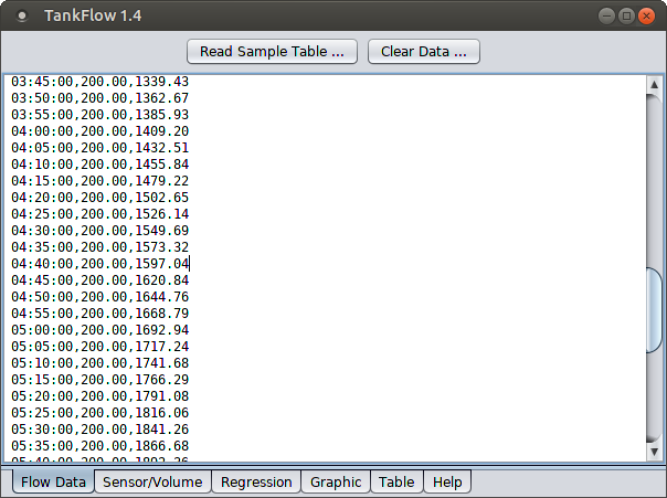
Figure 4: Flow Data tab
Now move to the "Sensor/Volume" tab and press the "Convert" button. The result should look more or less like this:
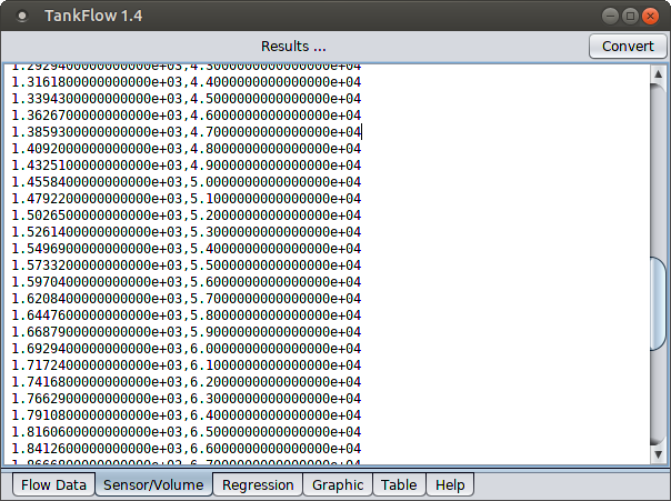
Figure 5: Sensor/Volume tab
This result shows that TankFlow has converted three-column field records (Figure 4) composed of times, flow rates and sensor heights into a two-column tank profile of sensor heights (Figure 5, left) associated with partial volumes (Figure 5, right).
- Even though TankFlow has converted the individual times and flow rates into a tank volume profile, there are only as many data points as field measurements, which leaves gaps in the predictive ability of the result table. In the next step TankFlow creates a continuous mathematical function to provide a sensor height for any desired volume (or the reverse).
Move to the "Regression" tab and press "Perform". The result shoud look more or less like this:
Figure 6: Regression tab
In this step TankFlow has converted a discontinuous list of volumes and sensor heights into a continuous mathematical function that can produce a sensor height for any volume, or the reverse. When program parameters are chosen carefully and assuming accurate field measurements, the resulting function can meet the most demanding accuracy requirements.
To test the accuracy of the result, move to the "Graphic" tab to see something like this:

Figure 7: Graphic tab (click for full-size)
The image in Figure 7 isn't large enough to show the full effect of the graphics feature (click the image for a larger version), but the red dots are the field measurements and the blue line is the trace created by the polynomial regression function. With care in data collection and processing, the mathematical function's trace will align with each of the field data points, showing that it accurately and continuously models the discrete data points, and therefore represents the sensor/volume relationship of the measured tank.
- TankFlow uses a mathematical method called Polynomial Regression to reduce field data and convert it into a more compact and useful form (more details below).
- TankFlow accepts field-recorded data as three-column records of times, flow rates and sensor heights, but it also accepts data of a more conventional kind — two-column records of tank volumes and corresponding sensor heights. To use TankFlow this way, paste the two-column data directly into the "Sensor/Volume" tab, then move to the "Regression" tab for analysis and function creation.
- The most important result created by TankFlow is the mathematical function created by the polynomial analysis, which can be exported and used anywhere — it's small, accurate and reliable. But for those who must have old-fashioned printed data, TankFlow includes a table generator at the "Table" tab. The resulting table can be copied to the system clipboard and used elsewhere. The "Table" tab includes controls to select start, end and step numbers to customize the table.
- To produce a mathematical function that accepts a volume argument and produces a sensor height (the opposite of the default), move to the "Regression" tab and enable the "Reverse x <-> y data" feature.
- TankFlow's analysis feature includes the most widely used metrics for evaluating results in this class — the "Correlation Coefficient" and "Standard Error" values. Ideally, the correlation coefficient value should be near 1.0 and the standard error value should be near zero.
- The graphic image displayed on the "Graphic" tab can also be copied onto the system clipboard for export — just press the "Copy Chart" button.
- In some cases the accumulated field measurements, and the regression method, produce a result that differs from the known lowest or highest volume of a tank, an outcome usually caused by a flow meter of limited accuracy. To deal with this case TankFlow includes adjustments to force the generated function into agreement with reality. To use this feature, go to the "Regression" tab, enter values in the "Correction Low" and/or "Correction High" entries, and enable these adjustments with the adjacent checkboxes.
- Apart from its primary purpose, TankFlow can perform general polynomial-regression analysis on user data entered into the "Sensor/Volume" tab. Its abilities match or exceed those of my popular online Polysolve polynomial regression application, with the advantage that TankFlow is a stand-alone application and has more ways to export its results.
- TankFlow provides a built-in sample data table for tutorial and instructional purposes ("Flow Data" tab, "Read Sample Table ..."). This table can be used to become familiar with expected data formats and to practice creating regression results.
- TankFlow saves all program information between uses — everything, including entered data. The data are saved in a user-level directory located at (user home directory)/.TankFlow. If problems arise and a fresh start is needed, simply delete this directory and run TankFlow again.
- To report bugs or ask for new TankFlow features, please visit this website's message board.
TankFlow addresses a common practical issue with storage tanks — many do not have documentation, and those that do, sometimes have unknown or pathological shapes that prevent a classical geometric analysis.
There are many tank shapes that can be characterized mathematically using these methods and equations and the assistance of a geometry-based program like my own TankCalc. But in practice, only some tanks fit into well-defined geometric categories. Some appear to be simple until one discovers some protrusion within the tank, or a distortion of shape or another reason that prevents a geometric treatment.
Calculus and rates of change
TankFlow addresses these problems by reducing a table of field measurements consisting of time, fill rate and sensor height into a stepwise tank volume profile. This method works because the flow of liquid into a tank represents a rate of change in the tank's volume. Those who have studied Calculus will know the meaning of the term rate of change — it means one may take that rate of change and integrate it over time to get a tank's partial volume at any given time.
TankFlow takes a table of field measurements, each having a time, flow rate and sensor height, and proceeds like this:
For each pair of records (call them A and B), TankFlow takes the provided flow rates and creates an average value equal to $\frac{A+B}{2}$:
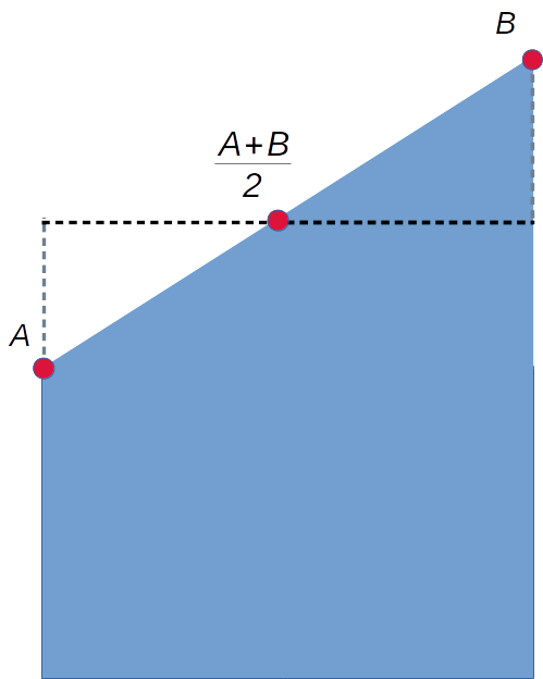
Figure 8: Computing an average value
A little geometric thinking reveals that this average value is exactly right if the flow rate changes in a linear way between A and B. If this is not true, if the flow rate value follows a curved path between A and B, then more data may need to be be collected to preserve accuracy.
- The flow rate computed in step (1) above is multiplied by the time interval between A and B. This volume change is added to the sum of past volumes to create an incremental tank volume at time B, associated with the sensor height recorded for time B.
- Steps (1) and (2) above are applied to all the field data to produce a complete stepwise tank volume profile correlated with recorded sensor heights. In essence, the recorded flow rates are numerically integrated to produce a stepwise volume profile for the tank.
The probem with this intermediate result is that it's incremental — there are gaps between volumes listed in the result. What we need is a continuous mathematical function to provide any sensor height for any specified volume, including volumes not recorded, as well as the reverse case (volumes for sensor heights). To get this result, TankFlow uses a method called polynomial regression (on the "Regression" tab) to convert the stepwise volume/sensor height table into a continuous function able to provide any volume for any sensor height or the reverse. The generated function can be exported into other environments and programs, and can be used to create a table of results with user-selected step sizes.
When generated carefully, the polynomial function serves as a very accurate model of the relationship between volume and sensor height, sufficient for any practical purpose. When fully exploited, the function does away with printed tables of values, guesswork, interpolation between known measured values and similar older methods.
Statistical Measures
The mathematical quality of the generated regression result can be gauged by examining the Correlation Coefficient and Standard Error values displayed on the "Regression" tab. The Correlation Coefficient value numerically describes the degree to which the regression result corresponds to the source data, and the Standard Error value provides a convenient gauge of likely errors in the results.
If these statistical measures don't meet requirements, there are some remedies. One is to increase the number and accuracy of the original field measurements, but this may require much time and effort. Another approach is to increase the "Polynomial Degree" value on the "Regression" tab, but this remedy has well-understood limitations — it can create a profile that perfectly matches the entered data at the measured points, but with no connection to reality anywhere else. Here's an example in which an attempt is made to use a polynomial regression technique to exactly match noisy field data:
First, copy this small data set into TankFlow's "Sensor/Volume" tab (second from left), while erasing any prior data that may be present:
-1 -1
0 3
1 2.5
2 5
3 4
5 2
7 5
9 4
- Directions: copy the above data by dragging your mouse pointer across the numbers, then press Ctrl+C (PC) or Command+C (Macintosh) to copy the data into the system clipboard. Then paste the result into TankFlow's "Sensor/Volume" by entering Ctrl+V (PC) or Command+V (Macintosh).
Now move to the "Regression" tab, select a polynomial degree of 2, and press Perform. Move to the "Graphic" tab to see this result:
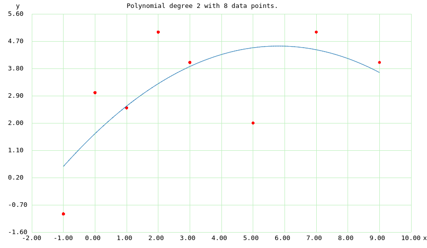
FIgure 9: Polynomial Degree 2, Correlation coefficient 0.4921, Standard Error 1.5179
Now return to the "Regression" tab, select a polynomial degree of 7, and press "Perform" again. The resulting chart should look like this:
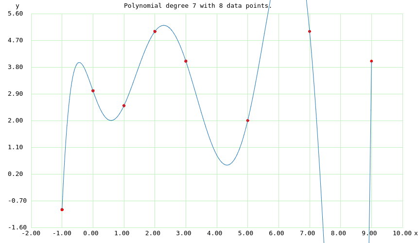
Figure 10: Polynomial Degree 7, Correlation coefficient 1.0000, Standard Error 0.0000
- The second result is statistically perfect, but meaningless.
In the above experiment, for polynomial degree 2, the regression doesn't agree with the data very well, simply because the data are so poor (or "noisy"). For polynomial degree 7, the regression matches the data exactly at each provided data point, but at the expense of having a pathological shape everywhere else. This shows the consequences of trying too hard to match noisy field data — the resulting analysis shows good statistical agreement with the data, but is otherwise useless and bears no relationship with reality.
The remedy for a case like this is to re-perform the field measurements — get better, more accurate data.
Flow Rate Accuracy
The process described above relies on minimizing systematic errors like time, sensor height measurement and flow rate. Flow rate in particular is a critical element of the analysis. For example, if the measured flow rates are in error by 10%, the tank's overall volume with be in error by this same amount.
TankFlow has a way to deal with this issue. For many tanks, their full capacity is known even though their content profile (Figure 7) is unknown. For a case like this, TankFlow applies a simple linear regression function to the generated incremental volume table, such that the profile is retained but all the values are adjusted so the low and high volumes agree with the correct values.
Here's the linear interpolation equation used by TankFlow:
\begin{equation} y = \frac{ (x-xa) (yb-ya) }{ (xb-xa) } + ya \end{equation}Where:
This deceptively simple equation can produce very useful results. For example, here are the values required to solve a temperature conversion problem:
- $x$ = argument in the $xa,xb$ range
- $y$ = result in the $ya,yb$ range
- $xa,xb$ = source numerical range
- $ya,yb$ = destination numerical range
- $xa$ = 32
- $xb$ = 212
- $ya$ = 0
- $yb$ = 100
Values $xa$ and $xb$ specify two known values on the Fahrenheit scale, while $ya$ and $yb$ are assigned the corresponding values in Celsius. If an argument $x$ is submitted in Fahrenheit, the equation will produce a $y$ result in Celsius. And a simple change in assignments can produce the reverse conversion.
In the context of TankFlow, if an inaccurate flow meter creates a table of sensor/volume results that has the right overall shape but the wrong specific values, this interpolation equation can be used to adjust all the values proportionally, thereby canceling out the flow rate errors while retaining the shape of the tank's height/volume profile. To get this result, the TankFlow user moves to the "Regression" tab, enters accurate low and high volume values in the "Correction Low" and "Correction High" windows, enables the adjacent check-boxes, and performs the regression again.
Set up this way, TankFlow uses the above equation to proportionally adjust the entire volume profile to create the expected low and high volume values, while retaining the overall shape of the profile (which is very likely to be correct).
Portable Results
Using the polynomial regression it creates, TankFlow draws a graph and allows creation of a table, but more importantly it provides a way to export a computer language function with appropriate polynomial terms for use elsewhere. On the "Regression" tab is a list of computer languages (top left). Selecting one of the languages generates a computer code function with correct syntax, ready for export via the system clipboard into another environment. Supported languages include C, C++, Java, JavaScript and Python.
One advantage to this function-export feature is that the result is much, much smaller than the tank's original data table. Another is that the function can portably recreate the tank's volume profile within any reasonable accuracy requirements. This allows TankFlow's results to find their way into user-created programs to, for example, print an old-style paper "strapping chart" for use in the field.
- 2019.07.04 Version 1.5. Added the ability to choose the number of decimal places in numerical results.
- 2019.07.04 Version 1.4. Added a quit button for platforms without window title bars, plus a few more small changes.
- 2019.07.03 Version 1.3. Redesigned the regression and chart tabs/interfaces for better, more intuitive operation.
- 2019.07.02 Version 1.2. Improved the graphic tab controls for better user interaction, included a sample data table for practice, cleaned up some minor bugs.
- 2019.07.01 Version 1.1. Fixed a few minor bugs, including one that sometimes prevented a successful start on Windows 10.
- 2019.06.30 Version 1.0. Initial public release.
| Home | | Mathematics | | * Applied Mathematics | | * Storage Tank Modeling | | | | Share This Page |