

 Share This Page
| Home | | Mathematics | | * Maxima | | | | Share This Page |
(double-click any word to see its definition)
This page shows an application of symbolic mathematics to the solution of an important real-world problem.
Some functions live alone in the world of mathematics, while others are more naturally organized into related sets. This project shows how a single equation can be used to construct a set of related equations. On this basis a set of functions can be created to solve an entire class of problems.
Future Value
In finance and banking, there is an equation that can be used to compute the future value of an annuity — not surprisingly it's called the "future value" equation. It has several variations. One variation arises from the fact that a payment into an annuity might be made at the beginning of the payment period, or the end. Two forms of the future value equation exist to take this distinction into account:
Equation (1), payment at beginning: 
Equation (2), payment at end: 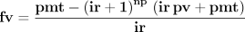
Where:
- pv = Present value of the annuity, the account balance at the beginning of the annuity term.
- fv = Future value of the annuity, the account balance at the end of the annuity term.
- np = Number of payments into the annuity during its term.
- pmt = Payment amount made during each period of the annuity.
- ir = Interest rate per period.
There are a few important things to be aware of when dealing with financial equations. One is that amounts withdrawn from an annuity have a positive sign, amounts deposited into an annuity have a negative sign. Adverse interest rates have a negative sign. Another important point is that the interest rate is per period, not per year or per term, so a 12% annual interest rate means 1% per period (assuming monthly payments), and the correct numerical value for 1% is 0.01, not 1.
Each of the above variables can be positive or negative numbers. A negative present value implies a deposit made at the beginning of the annuity's term. A negative payment amount implies a net inflow of cash during each period. A negative interest rate implies an interest deduction from the account's balance each period. Here is an example annuity computation:
- pv = 0
- np = 120
- pmt = -100
- ir = 0.01
These values describe an annuity such as an investment, with a favorable interest rate of 1% per period, a deposit of 100 currency units per period, and 120 payment periods. For these values, and assuming payment at the end of each period, the future value will be 23,003.87 currency units (rounded to the nearest 1/100). For the case of payment at the beginning of the period, the future value will be 23,233.91 currency units. The reader can check these results using a spreadsheet program, most of which have an FV() function available. Here are typical spreadsheet entries for this problem:
=FV(0.01;120;-100;0;0) 23,003.87 Payment at end. =FV(0.01;120;-100;0;1) 23,233.91 Payment at beginning.
The Goal
Now that we've established the preliminaries, let's state a goal. In this project we want to create functions for each of the variables in the future value equation, so we can solve for any value in an annuity. And it would be nice to be able to deal with the issue of payment at beginning or end without having to write two sets of equations.
The first step in our project is to create a meta-equation that accommodates the issue of payment at beginning or end. The new equation deals with this issue by including a new variable pb that makes the equation switch between modes. This part of the project isn't strictly speaking about Maxima, since it requires a kind of analysis not likely to be available to a symbolic math program — but on the other hand, we can check the outcome using Maxima, to be sure the idea works.
Here is the meta-equation:
| (3) |
|
Here is a line of text the reader may use to enter this equation into wxMaxima (copy the entry from the display):
eq:fv=((pb*ir+1)*pmt-(ir+1)^np*((pb*ir*pmt)+pmt+ir*pv))/ir;
Now for a sanity check. Can we derive the two forms of the future value equation from this meta-equation, simply by setting the value of of the variable pb? Let's see:
eq; (let's check to see if the equation was read correctly)
pb:0; (set pb = 0, meaning payment at end)
ev(eq); (use "evaluate" to interpret the equation)
pb:1; (set pb = 1, meaning payment at beginning)
ev(eq); (use "evaluate" to interpret the equation)
Perfect result.
A technical note. A variable that assumes values of zero or one can be used as a switch, in effect adding or removing terms from an equation. The function "ev()" simplifies equations that are submitted to it, and in this case, if the pb variable is set to zero, "ev()" eliminates any terms that are multiplied by it. If the pb variable is set to one, the "ev()" function retains the associated terms and eliminates only the pb variable itself.
The meta-equation in essence recreates the two canonical forms of the future value equation, and applying the "ev()" function proves this. But it's important to note that, even without this term elimination, the original meta-equation will still deliver correct results if the pb variable is set to zero or one to convey the user's intentions.
This idea seems to be successful — setting the value of the pb variable in the meta-equation appears to recreate the two original forms of the future value equation. This will greatly reduce the number of required equation forms and the overall complexity of the project.
Now we can create all the forms the future value equation can take, based on the variables within it. First, some keyboard entries to make sure this approach will work:
kill(pb); (remove any assignment to pb)
eq; (is our equation still present?)
sol:solve(eq,pv); (solve for variable pv, present value)
rhs(sol[1]); (isolate the body of the solution for use in a function declaration)
Okay, it seems we can create versions of the meta-equation to provide results for each of the variables in the original equation. Let's write a function that automates the process of solving for specific variables and isolating the desired expression:
solve_for_var(eq,v) := ev(rhs(solve(eq,v)[1]),fullratsimp);
The reader will appreciate that I have skipped over a few details in the design of this function. The "solve_for_var()" function solves for a particular variable, isolates the required expression, prepares it for assignment to a function description, and simplifies it ("fullratsimp") if possible. Such a function has the advantage that its actions are encapsulated, they don't have to be entered repeatedly, and further, if a change is made to the algorithm, the change only needs to be entered in one location to have an effect on all the derivations.
Having written a function to create equations for each of the variables, we can now simply and quickly produce all the desired functions:
fpv(fv,np,pmt,ir,pb) := solve_for_var(eq,pv);
ffv(pv,np,pmt,ir,pb) := solve_for_var(eq,fv);
fnp(fv,pv,pmt,ir,pb) := solve_for_var(eq,np);
fpmt(fv,pv,np,ir,pb) := solve_for_var(eq,pmt);
fir(fv,pv,np,pmt,pb) := solve_for_var(eq,ir);
NOTE: The interest rate case isn't soluble in closed form, and the function declaration is only present for completeness ... and a tiny penchant for mischief. More below.
At this point it should be apparent that this sort of detailed processing is much more efficiently placed in a file to be loaded and executed by Maxima. Here is a link to the file. When loaded into Maxima using "batchload()" as shown earlier in this article set, the four derived functions will be created and listed, and two example computations will be performed and displayed, for future values with payment at beginning and end for the problem statement provided above.
Even though there is a derivation for "ir", the interest rate, it turns out this case is not soluble in closed form, as Isaac Newton discovered in his second career as Chancellor of the Exchequer, during which time he applied his substantial mathematical gifts to the mundane problems of finance. I only include the derivation to reveal something about symbolic math packages — on occasion they will very happily produce meaningless results. And if the resulting function is tested, it will ... well, how shall I say this? ... go completely nuts. Try it:
fir(23003.87,0,-100,120,0);
(huge display of garbage results)
The reason for the crazy behavior? Simple — "solve()" didn't really solve this one. The result created by "solve()" has "ir" terms on both sides of the equals sign. I would have been happier with an error message, but no symbolic math packages are perfect, and Maxima is, after all, free. In normal practice, computing interest rates involves a root finding approach using another form of the equation (see my Finance Calculator page for a practical embodiment).
| Home | | Mathematics | | * Maxima | | | | Share This Page |