Introduction
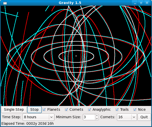
Typical display — best viewed with anaglyphic glasses ( ).
).
Since the day I got my first computer in 1977 (an Apple II), I've been writing gravity simulators, and until now they've been rather difficult to create and test. But I recently learned Ruby, and I must say that, given how sophisticated this new simulator is, I am astonished at how quickly it came together. Even though I have ported this simulator to C++ for greater execution speed, I am glad I designed it in Ruby first, because of the startlingly short prototyping and development time.
This gravity modeler operates in three dimensions (a personal first), and it shows its results in true 3D using the anaglyphic method (using red/blue glasses). It was written and tested on a Linux system, but it will run on Windows if Ruby and the GTK+ library are installed.
In brief:
|
Name:
|
Gravity, version 1.5 (12/01/2008). Distributions for both Ruby and C++.
|
|
What it is:
|
A sophisticated, three-dimensional physical simulation of orbital dynamics with fast animations and 3D (anaglyphic) rendering capability.
|
|
Written in:
|
Ruby 1.8.4. (then C++, after being designed in Ruby)
|
|
Requires:
|
The GTK+ library, version >= 2.0 and Ruby, version >= 1.8. Both GTK+ and Ruby are free, cross-platform and open-source.
|
|
Objects:
|
Nine planets, plus a user-selected number of rogue comets (see picture this page).
|
|
Optional, very desirable:
|
Anaglyphic glasses () to see the 3D effects.
|
|
Source:
|
Ruby interpreter files: rubygravitation.zip (10 KB).
C++ source package: gravity.tar.bz2 (215 KB) or an exectable binary created on Fedora 10 (200KB).
|
|
License:
|
GPL.
|
In this article I'll describe the mathematics and physics behind this kind of modeling, and I'll discuss some of the programming issues.
The Physics of Gravitation
We're all indebted to Isaac Newton for sorting out the first set of mathematical rules for gravitation. Albert Einstein added a great deal to our understanding of gravity, but in normal circumstances Newton's equations can be used to predict gravity's effects in nature.
The first thing to understand about gravity is that its "force"
1 declines as the square of distance:
| (1) f ≈ | 1 |
 |
| r2 |
So, if you double the distance between two masses, the gravitational force declines by a factor of four. A full statement of the force of gravity is that it is equal to the product of the masses and a gravitational constant G, divided by the square of the distance between the masses:
| (2) f = G | m1 m2 |
|
| r2 |
Where:
|
f:
|
Force, Newtons, and please read footnote 1.
|
|
G:
|
The Universal Gravitational Constant, estimated to be equal to 6.6742x10⁻¹¹ N m2 / kg2.
|
|
m1,m2:
|
The masses of the two bodies in question.
|
|
r:
|
The distance between m1 and m2.
|
All in consistent units.
We have the force, but there is one more step in moving one of the masses, and that is to apply the force. When we apply the force, we discover something Einstein showed us — masses posses inertia, and further, inertial mass and gravitational mass are equal (as far as can be determined).
Therefore, to convert a force to an acceleration, we apply this equation:
| (3) a1 = | f |
|
| m1 |
Well, well. It turns out that acceleration (the rate of change in velocity) is inversely proportional to mass. But the force of gravity is directly proportional to mass, therefore two mass terms cancel out — one mass term in equation (2) and one mass term in equation (3). In some cases we can combine equations (2) and (3) like this:
| (4) a1 = G | m1 m2 |
|
m1 r2 |
Canceling terms:
| (5) a1 = G | m2 |
|
| r2 |
Equation (5) is suitable when mass
m2 is much greater than
m1, such as the problem of a planet traveling around the sun.
At this point we've established the force between two masses at rest, what is known as a "static problem". You can measure the force with reasonable accuracy, then you can move the masses, then you can measure the force again. But in nature, masses tend to be in continuous motion. How can we predict the future path of a moving object under the influence of gravity? Aren't the forces changing from moment to moment, making it tough to do the math?
There is a tool that is perfectly suited to this kind of problem. It's called "Calculus". I have written a
tutorial on Calculus for those who want a quick refresher before we go on. It turns out that Calculus, the mathematics of motion and change, is the perfect tool for gravity simulation.
A Little Calculus
Those of my readers who haven't studied Calculus shouldn't worry — the graphics will likely convey the key ideas, and I will do my best to explain the concepts as we proceed.
At this point, we are going to allow our masses to move, and if we intend to model that motion mathematically, we need a way to put motion terms in an equation. Let's say we have a function
2 that tells us where we are at time
t, and it looks like this:
(6)
p(t) = v t
Very simply, function (6) says, "Position
p(t) at time
t is equal to a velocity term
v times
t". If our velocity
v is equal to 5 meters/second, then according to function (6), after 23 seconds we should have moved 23 * 5 = 115 meters.
Differential Equations
We know what is in
p(t) above, what operation it performs, because we stated it explicitly. But there is a reason to treat functions as though they were variables, black boxes with just a name, boxes that can contain anything at all. We know we can make statements about numerical variables without knowing or caring what the variables contain, indeed that is the primary idea behind algebra. It turns out we can make statements about functions in the same way, without knowing or caring what the function actually does.
Because we know what is in
p(t) above, we know there is a velocity term present. But let's say we need to refer to velocity if given a position function with unknown contents. Using
differential equation notation, we can say:
(7)
v(t) = p'(t)
Our new function
v(t) represents the
rate of change in the position function
p(t), with respect to time
t. We specify a function's derivative (a rate of change) with the notation in (7), that is,
p'(t).
Again, this is a simple notation, it's useful and important to remember. It simply says that
p'(t) is the
rate of change in
p(t). If p(t) happens to refer to a position at some time
t, then
p'(t) refers to the rate of change in position, or velocity (or speed, for purists).
Higher derivatives
If
p'(t) is a rate of change in
p(t), and
p(t) is a position at some time
t, then what might
p''(t) signify? Strictly speaking, that would be a
rate of change in a rate of change with respect to
t. And if
p'(t) is a velocity, then
p''(t) must refer to acceleration, which is defined as a rate of change in velocity. Or:
(8)
v(t) = p'(t) (velocity from position)
(9)
a(t) = v'(t) (acceleration from velocity)
Of course, we can take this shortcut:
(10)
a(t) = p''(t) (acceleration from position)
Ball, Dog, Wind
At this point we can use this notation to make a rather sophisticated statement about a physical problem. Let's say we have thrown a ball into the air. We have released the ball with an initial velocity v at time zero, and we want to know where the ball will go under the influence of gravity. We'll disregard such factors as air resistance, the neighbor's dog, and all those messy real-world factors that mathematics doesn't address very well anyway.
Here we go. We've thrown the ball, let it go with a starting velocity of
v at time zero. We want to make a statement about how gravity will affect the ball. First, let's figure out what force Earth's gravitational field will create on the ball (a restatement of equation (2)):
| (11) f = G | m1 m2 |
|
| r2 |
In this case,
m1 is our ball,
m2 is the Earth (a bigger ball), the radius
r is the distance from the center of the earth to the surface
3, and
G is the Universal Gravitational Constant. Here are the values:
|
Mass of the ball (m1)
|
250 grams
|
|
Mass of the Earth (m2)
|
5.976x1024 Kilograms
|
|
Radius of the Earth (r)
|
6.37814x10⁶ Meters
|
|
Universal Gravitational Constant (G)
|
6.6742x10⁻¹¹ N m2 / kg2.
|
Plugging in these numbers:
| (12) f = 6.6742x10⁻¹¹ (G) | .25 (ball) 5.976x1024 (earth mass) |
|
| (6.37814x10⁶)2 (earth radius) |
Before going on, remember equation (5) above, that cancels out two terms and gets us to acceleration in one step? Let's apply that simplification:
| (13) a = 6.6742x10⁻¹¹ (G) | 5.976x1024 (earth mass) |
|
| (6.37814x10⁶)2 (earth radius) |
Our result is an acceleration of about 9.8 meters/second
2 (that's about 32 feet/second
2 in English units), a number that should be familiar to many people in technical professions.
Now let's write a statement about the ball's flight, using the notation we have introduced above:
|
Term
|
Meaning
|
Comment
|
|
p(0) = 0
|
Initial position at time zero
|
The position of the thrower's hand releasing the ball
|
|
p'(0) = v
|
Initial velocity at time zero
|
The velocity imparted to the ball by the thrower
|
|
p''(t) = -a
|
Gravitational acceleration
|
A constant for any time t
|
These items are called "differential equation terms." They may or may not lead to a closed-form solution, an ordinary algebraic function for any time
t. As stated, they do in fact lead to a trivial solution, because there are only two gravitating bodies involved (and because we chose to neglect wind and the neighbor's dog):
Plot for a = 9.8, v = 19.6
| (14) p(t) = - | a t2 | + t v |
|
| 2 |
About equation (14), notice the
-a t2/2 expression? That's what makes the ball come back down. The expression to its right,
+ t v, initially causes our thrown ball to travel upward, but the time-squared term eventually dominates.
If a closed-form solution were not available, if this problem represented a physical system that could not be solved algebraically, there would still be options. One commony used option is to model the system in small slices of time. This is called "numerical modeling". Obviously it would be better to find a closed-form solution, since that would produce an immediate result for any time, with very little computer power expended. One applies numerical solutions only as a last resort.
This leads to a famous question. How many gravitationally interacting bodies can you have, and still produce a closed-form solution? The answer is "two". This means the problem I stated above is the most complex form that avoids labor-intensive numerical methods. All other problems in this class require numerical modeling.
So when you hear that NASA expended vast sums guiding a Mars lander spacecraft from Cape Canaveral, using exquisitely accurate methods, over many months of deep space flight, to a point 80 million kilometers away, where the spacecraft crashed only a few meters from its intended touchdown point, you should remember they used methods very much like those used in my modeling program.
Programming Calculus
We have established that a general-purpose gravity simulator must compute its results numerically, that is, in steps, using many small slices of time. This approach has a number of advantages, the most important being a simple statement of some rather complex problems, but it has these drawbacks:
- From the standpoint of accuracy, it is a good idea to use small time slices, but computer numeric variables have limited resolution, so we must avoid making the time slices too small. Also, small time slices mean long execution time.
- From the standpoint of fast execution, it is a good idea to use large time slices, but a numerical algorithm's results become less accurate as the time slices become larger.
These two points are obviously in conflict, and a reasonable numerical solution balances the issues of accuracy and execution time. But it is important to understand that
all numerical solutions are approximate. One can minimize computation errors, but they cannot be eliminated.
Here is an example numerical solution for a problem whose result we know, so we can evaluate the difficulties. Above, we had expressed the idea of throwing a ball into the air, and discovered that there is a simple algebraic solution. For this exercise, let's try solving that problem numerically and see where it takes us.
Here is a method, written in Ruby, that numerically solves the ball-throw equation:
def numeric_solve(dt,v,a)
   t = 0
   p = 0
   max = 0
   while p >= 0
      v += a * dt
      p += v * dt
      t += dt
      max = p if p > max
   end
   return t,max
end
For this method, we provide arguments for a time interval (dt), an initial velocity (v) and a gravitational acceieration (a). From a Ruby program, we might call the method like this:
numeric_solve(.001,19.6,-9.8)
In the Ruby simulation program (
HTML/
plain text), I got these results for different
dt values:
dt:  0.100000 height: 18.620000 error %: -5.263158 runtime:  0.000139
dt:  0.010000 height: 19.502000 error %: -0.502513 runtime:  0.001019
dt:  0.001000 height: 19.590200 error %: -0.050025 runtime:  0.012192
dt:  0.000100 height: 19.599020 error %: -0.005000 runtime:  0.122441
dt:  0.000010 height: 19.599902 error %: -0.000500 runtime:  1.188301
dt:  0.000001 height: 19.599990 error %: -0.000050 runtime: 11.969762
These results were obtained on a relatively fast PC with a 3 GHz clock speed. From the algebraic solution above, we find that the maximum ball height should be 19.6 meters, so in our simulation we've used that result as a measure of the accuracy of the numerical solution. This experiment shows us several things:
- Within broad limits, reducing the size of dt (the time slice value) proportionally reduces the numerical error.
- Numerical solutions can take a long time. This problem is typical in that each decimal place of accuracy improvement requires ten times more computer time.
- Minimizing errors in numerical solvers quickly become a case of diminishing returns. In the above example, the worst-case run time for the simulation took longer (12 seconds) than the ball throw would have required in reality (4 seconds).
- Not demonstrated in this solution is the fact that, for some problems, reducing dt too far backfires (because of roundoff errors in the computer's floating-point variables), and the errors increase again.
This would seem to have been a rather masochistic exercise, since we already know an algebraic solution exists. But in physics, the vast majority of dynamic problems require numerical solution, so it is a good idea to learn how to perform these kinds of simulations, and avoid the pitfalls.
Simulating Space
Now we can turn to the full-fledged gravity simulator. As explained above, the program is written in Ruby, which was a tremendous advantage with regard to develoment time. I was able to move from a rough outline to final code is a very short time.
To run the program, follow these steps:
- Download the ZIP archive rubygravitation.zip
- Unzip it into any convenient directory:
$ unzip rubygravitation.zip
- Run gravity.rb:
$ ./gravity.rb
Remember that you must have installed the GTK+ Library and Ruby itself (see top of this page for links). If you are on a Linux platform, this will be either true already or easily done.
Once the program is running, press the button marked "Run" to start the default animation, which consists of the solar system's nine planets.
- To zoom out to see the outer planets, put your mouse cursor in the space view window and spin the mouse wheel.
- To change the angle of view, drag the mouse cusor in the space view window.
- To see true 3D, click the "Anaglyphic" check box, and put on your anaglyphic () glasses.
- To add some random comets on highly elliptical orbits (typical for comets), click the "Comets" check box.
- To allow the orbiting objects to leave trails in their wakes, click the "Trails" check box.
The default time step (think
dt from the above examples) is 16 hours, which makes the inner solar system's planets seem to be moving rather fast (if your system's clock speed is also fast). If you reduce the time step, the simulation will be more accurate, but it will take longer to run. If you increase the time step, the animation will go faster, but wil be less accurate, as explained above.
When very large time steps are selected, the simulation will go out of control and some planets will depart the solar system at high speed. To recover from having destroyed the solar system, reduce the time step to a reasonable value, then click the "planets" check box twice, which reloads the original solar system positions and velocities.
If you maximize the program's window, the orbital display will be scaled up to accommodate the larger display area, and the simulation will run at a slightly slower rate. If you have a very fast system, you may want to try increasing the number of comets, but this slows the simulation down rather severely.
Program Notes
For those who are interested,
click here to see the main Ruby program listing (it can't be run stand-alone, it requires additional files present in the
zip download).
As I developed this simulator, I decided to include some real-world orbital data, to see if the resulting simulation agreed with reality. So I acquired a table of solar system data (planetary positions and velocities) and included it in the program. I realized I had written a valid simulation when the planets didn't fall into the sun.
As to the comets, I wrote a random comet generator (each new set of comets is different) that creates reasonable-looking elliptical orbits. Obviously this program's frequency of inner-system comet encounters is higher than in reality.
The user will notice that, even with a time step of 1 hour, Mercury seems to be orbiting the sun rather quickly. This is because each simulation "hour" may take only a few milliseconds to compute and render. Watch the time display at the lower left to see how quickly time passes in the simulated world.
The simulator's solar system representation is only approximately correct. In the real world, not all the planets lie on the same plane. A user with some programming skill could create a data table for the solar system that includes much more detailed information, such as inclination to the ecliptic and accurate planetary positions for a given starting date.
The reader may know that orbital systems with more than two bodies are potentially chaotic (e.g. extremely sensitive to initial conditions and prone to unpredictable instabilities). The only reason we don't notice this in our own (real-world) solar system is because the sun's mass is so much greater than the planets that each planet represents an individual two-body orbital system with the sun.
Symmetrical Gravity Computation
In the real world, each mass interacts gravitationally with every other mass, something that is easy to say but hard to model in a computer. If we wanted to maintain perfect fidelity to reality, we would compute each object's gravitational acceleration toward every other object, which unfortunately requires time proportional to n(n-1)/2 for n objects. In this simulator, both to assure stability and to save time, the gravitational accelerations of the planets and the comets are by default computed with respect to the sun, not to each other.
But there is an option in the program that can compute all the objects symmetrically. Located in the
source listing at
OrbitalPhysics::process_planets, this approach proves useful in simulations other than those provided by default with the program (and only in a much faster execution environment than a typical P.C.). An example would be a star cluster, a notoriously difficult system to model, and one that would require a fantastic amount of run time on a personal computer. This option is available for code completeness but it isn't practical to use in the Ruby version of this program.
C++ Version of Gravity
It is because of modeling challenges like star clusters and my curiosity about the above-referenced symmetrical computation mode that I have written a version of this program in C++ to improve execution speed. This version is available as a tar archived source package that must be compiled for use, and it is meant for a Linux system having an installed GTK+ library.
Click here to download the C++ source package (215 KB), or
click here to download a binary executable compiled on Fedora 10 (200KB). As expected, the C++ version is much faster than the Ruby version, and it reveals some things I didn't expect. One of these is that graphically rendering a huge number of "comets", a program option, takes much more processing time than simply computing their path through 3D space. I discovered this by reducing the minimum size of the objects ("Min. Size") and seeing a dramatic increase in rendering speed.
The C++ version will readily draw many thousands of objects with acceptable speed, and presents quite a spectacle when the render is carried out using the 3D anaglyphic rendering option. To create thousands of objects, simply choose a large number of "comets" from the provided drop-down list. This mode of operation really shows the downside of Ruby in execution speed. The Ruby version will run acceptably fast only until there are about 16 objects present, after which it begins to slow down severely.
This is not meant to disparage Ruby, not at all. This is not what Ruby was designed to do. And Ruby allowed me to develop this application very quickly (another meaning for program speed), after which I simply ported the program, almost line by line, into C++.
Revision History (Ruby and C++)
- 12/01/2008, Version 1.5. Overhauled both versions (Ruby and C++) of this program to eliminate use of the Qt library, replacing it with GTK+.
- 09/19/2006, Version 1.4. Replaced rotation matrix with a faster one that doesn't support rotation around an unused axis.
- 09/15/2006, Version 1.3. Refactored some time-critical code sections.
- 09/15/2006, Version 1.2. Further optimized after writing C++ version.
- 09/15/2006, Version 1.1. Optimized some sections of the code.
- 09/14/2006, Version 1.0. Initial Public Release.
Footnotes:
1. Gravity isn't really a force according to General Relativity, but please accept my use of this everyday term.
2. A function is a named abstraction that represents one or more mathematical operations. It accepts one or more arguments and produces a result. A named function is to mathematical operations what a named variable is to numbers.
3. It turns out that planetary gravitational calculations can be carried out using the simplifying assumption that all the mass is concentrated at the center of the planet. So we proceed as though we are some 6000-odd kilometers away from an extremely dense object.

 Share This Page